Statistical techniques for handling high content screening data
Posted: 21 September 2007 | | No comments yet
One of the chief incentives for the use of high content screening (HCS) approaches is the data rich return one gets from an individual assay. However, conventional methods for hit selection and activity determination are not well suited to handling multi-parametric data. Tools borrowed from the genomics area have been applied to HCS data, but there are important differences between the two data types that are driving the development of novel statistical approaches for HCS data analysis. This article will describe the use of techniques such as principal component analysis, classification trees, neural networks and random forests, as well as recently published approaches for the identification and classification of compound profiles resulting from HCS assays.
One of the chief incentives for the use of high content screening (HCS) approaches is the data rich return one gets from an individual assay. However, conventional methods for hit selection and activity determination are not well suited to handling multi-parametric data. Tools borrowed from the genomics area have been applied to HCS data, but there are important differences between the two data types that are driving the development of novel statistical approaches for HCS data analysis. This article will describe the use of techniques such as principal component analysis, classification trees, neural networks and random forests, as well as recently published approaches for the identification and classification of compound profiles resulting from HCS assays.
One of the chief incentives for the use of high content screening (HCS) approaches is the data rich return one gets from an individual assay. However, conventional methods for hit selection and activity determination are not well suited to handling multi-parametric data. Tools borrowed from the genomics area have been applied to HCS data, but there are important differences between the two data types that are driving the development of novel statistical approaches for HCS data analysis. This article will describe the use of techniques such as principal component analysis, classification trees, neural networks and random forests, as well as recently published approaches for the identification and classification of compound profiles resulting from HCS assays.
High content screening (HCS) is becoming an increasingly popular format for the early identification of biologically active compounds. The attraction of HCS assays is that they give flexible and comprehensive data on compound effects in a biologically relevant setting, typically the cell. Diverse responses such as changes in protein expression, activation, ion fluxes and cytotoxicity can be monitored, in some cases simultaneously.
Commonly, but not exclusively, HCS is applied at the secondary screening or lead optimisation phase of pharmaceutical development. At this stage, obtaining a rapid and in depth assessment of the cellular effects of a compound is invaluable in selection of compounds or series for progression. HCS is ideally suited for this purpose since the application of automated imaging and analysis algorithms can report a multitude of on-target and off-target responses in a single assay.
Although HCS has been integrated into many lead selection campaigns within the industry, the data that results from a HCS screen differs from that of “conventional” assays. Where a conventional assay may report one or two data points per well, a HCS assay may report one hundred or more. With the increased through-put of the latest HCS readers, and more advanced imaging algorithms available to the user, handling, manipulating and interpreting the data represents a significant and novel challenge. Fortunately, several recent publications and software products are providing the tools necessary for informed compound selection.
Primary data inspection
The statistical approaches for hit selection from high through-put screens have been well established1. Typically, a compound is classified as active if its signal lies outside a threshold value (normally determined as a number of standard deviations away from the median signal of the negative control). Whilst this approach can work well as a first pass for HCS data it ignores the breadth of information that can be derived from a HCS assay. Other parameters derived from the image can refine hit selection to give more accurate identification of active compounds.
Figure 1.a shows the results of 60,000 compounds assayed in a fluorescent cell based HCS for receptor internalisation2. As in a conventional screen, initial analysis focused on one parameter for hit identification. Compounds identified as hits are shown in red. However, the images were also analysed for a number of other cellular features relating to the intensity and localisation of fluorescence within the cell representing over 20 different parameters. How can these additional features be used to refine hit selection to identify the true positives?
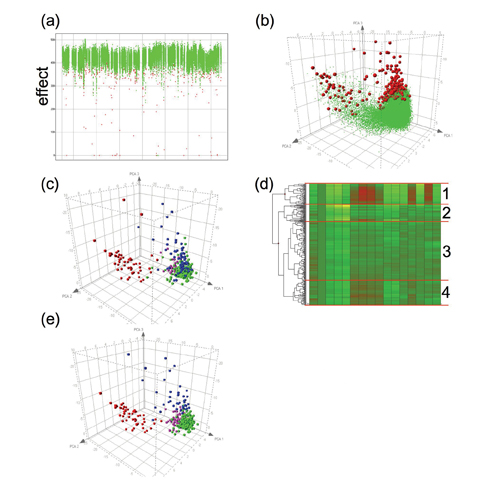

Figure 1: Results of a primary HCS screen. (a) Hits (red) are identified from non-hits (green) by a single parameter; (b) PCA of multiple parameters shows two distinct classes of hits; (c) Replotting of the hits and classification by visual inspection of toxic compounds (red), imaging errors (blue), fluorescent compounds (pink) and true hits (green); (d) Hierarchical cluster analysis of the data from the hits shows 4 distinct clusters; (e) Recolouring of the PCA plot according to cluster (1, red; 2, blue; 3, green; 4, pink) shows a close resemblance to visual classification in (c).
The simplest approach to refine hit selection is just to apply multiple selection thresholds to the data. For example, invariably some compounds used in the screen will cause cytotoxicity, which may manifest itself in a reduction in the cell number. So we can filter on those wells with a low cell number to reduce the incidence of toxicity related false positives. Alternatively, the compound may be fluorescent itself, therefore interfering with the marker signal. Filtering out wells that contain very bright or very dim fluorescence cells can further reduce false positives.
One drawback of this above approach is that prior knowledge of the types of false positives that may arise is required. Other drawbacks include the fact that the analysis is still reliant on a small subset of data generated as opposed to using all the information available and the application of multiple hard thresholds increases the risk of misclassifying a true positive compound.
A common method for investigating multi-parametric data is principal component analysis3 (PCA). PCA is primarily a dimension reduction technique, which enables the variation seen in many different parameters to be encapsulated in the minimum number of values. Principal components are the sum of individual measurement parameters multiplied by different weighting factors.
By performing PCA on the dataset in Figure 1.a we can start to visualise all the data resulting from the multi-parametric analysis of the images (Figure 1.b). The majority of the compounds sit in a “cloud” towards the bottom right of this plot. These compounds are having no significant effect on the measured parameters. The compounds classified as being hits (red) fall roughly into two areas; the first is plotted towards the top of the main group of compounds and separates from the no-hit cloud by having a more negative value on the 3rd principal component axis. The second hit grouping is directed towards the left of the plot. This group is linked to the main no effect cloud by a tail of compounds classified as non-hits but separated from the bulk of the compounds.
By visual inspection of the images relating to the compounds classified as hits (Figure 1.c) we can quickly identify that the lower middle group contains the majority of true hits (shown in green), whereas the upper left grouping contains cytotoxic false hits (red); this also suggests that the non-hits in the tail region in Figure 1.b may be cytotoxic too. Other classes of false positives also start to group together such as imaging errors (blue) and fluorescent compounds (pink). The PCA plot enables the identification of the compound group that contains the highest likelihood of being a true hit compound.
Compound groupings can be analysed by a variety of cluster analysis routines, such as K-means clustering, self-organising maps and hierarchical clustering3-4. Each of these approaches aims to group datasets with similar profiles across all the measured parameters. Figure 1.d shows how the most commonly taken approach, hierarchical clustering, groups the data from Figure 1.c. The clearest separation is between a group containing the majority of the compounds causing toxicity and the remainder of the compounds, but other groupings are apparent. Re-colouring the PCA plot from Figure 1.c by membership of the 4 largest clusters (Figure 1.e) shows how cluster analysis mirrors the classification by visual inspection. These quick and simple tools enable rapid identification of the true hits and false positives without the need for laborious and subjective manual image inspection.
Supervised models
A second approach to classification of hits is to use supervised models. In general these models use a subset of validated data as a training set with which to build “classifiers” based on the measured parameters. In practise the training sets would be a small sub-screen of compounds with known biological response, be it active, inactive or causing an off-target effect such as toxicity. Training sets can also be built from data where images have been manually inspected.
Several different methods can be used for supervised models. Perhaps the simplest is the decision tree method5. Here the model is based on a branching set of tests, each one dictating which subsequent test to apply. The model keeps applying different criteria to split the dataset until the data that lead to a common branch are homogenous, or of the same class. In effect the repeat application of filters to remove false positives described above is a simple example of a decision tree model.
For various reasons, decision trees have limited usefulness since the models can be sensitive to the selection of the training set of data. A development of decision trees, called random forests6 can address this issue by building many decision trees based on a random subset of the data. The multiple decision trees increase the robustness of the model, and classification of a test set of data is done by analysing the most common classification from the forest of decision trees.
Another popular classification approach is the use of neural nets7. These models mimic the way that neurons rely on a number of inputs to dictate whether they fire or not. Neurons initially fire in response to the data set then the signal is propagated through the network of neurons which results in a final classification result. Models are built to optimise the correct classification of the training set and then test data is applied to the network. Neural nets can often perform well at classifying HCS data but have the drawback that it is difficult to de-convolute how and why a particular classification was made.
A third method for distinguishing different classes within HCS data is the use of linear discriminant analysis (LDA)8. Unlike the two methods above LDA has a mathematical, rather than stochastic, basis for classification. The approach used in LDA is similar to that for PCA, but whereas PCA describes the factors which contribute to the variation seen across all the data, LDA identifies the combination of parameters which best describe the differences between data sets belonging to different classes.
As an example of how these different approaches perform, Table 1 shows how the data from Figure 1 are classified using four different approaches. In each case a subset of data that had been verified by visual inspection was used to build the models and then the remainder of the data was then classified by the models as being true hits or false hits. Model performance was assessed by counting the number of false classifications, confirmed visually, made by each model.


The first model is based on repeated application of individual thresholds for selection of true hits. Whilst this does reduce the number of false hits, the number of misclassified true hits – representing active compounds that would be rejected was high. The three other models based on random forests, neural nets and LDA each out-perform the simple rule-based approach and offer a more accurate way to classify the data.
In practise, it is likely that different approaches will be better suited to different biological assays used in HCS. Classification models are likely to be more robust and out-perform rule-based methods. In our experience, classification models have led to the identification of a number of true hits that have been missed by conventional hit selection methods. The reason for this is that they are based on multiple parameters from the HCS data and are therefore less prone to the misclassification of true hits; probably the most serious error is screening data analysis. In building models by each of the three above approaches it is possible to weight the importance of misclassifications, thereby reflecting their true severity in compound selection9.
Secondary screening approaches
Many of the approaches outlined above would be familiar to those who regularly handle genomic data. In many respects data from HCS screens is reminiscent of that from the genomics field. However there are important differences. The first is that HCS data tends to be “taller”, (for example, 10,000’s of conditions) and thinner (for example,100’s of parameters) than genomic data which is typically composed of 10’s or 100’s of conditions and 10,000’s of genes. With genomic data the main question is to identify which genes respond to a particular condition and use these to characterise the biological response. With HCS data we commonly want to identify which conditions give a desired biological response, so there is a shift in emphasis when the aim is to classify conditions rather than genes.
A second difference is in the inter-related nature of the data points. A pharmacologist is interested in dose response relationships, rank ordering of potency and windows of activity. Due to the nature of data, dose relationships are rare in genomic data. Since many HCS screens are directed at the secondary or lead optimisation phase of drug discovery then there is a clear need for HCS approaches.
To interpret dose relationships within HCS data we can use principal component analysis as a preliminary visualisation tool. Figure 2 shows the result of a cell based imaging assay to identify compounds that cause accumulation of phospholipids within cells. Cells were exposed to a number of compounds across a dose range and then imaged. These images were then analysed using algorithms to report both the accumulation of phospholipid, but also general cell morphology. Principal component analysis was performed on these features and the 3 principal components are plotted.
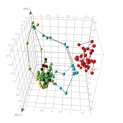

Figure 2: Dose response relationships visualised by PCA. Positive (red) and negative (green) controls from a cell based assay are plotted alongside dose responses for 3 different compounds. Compound 1 (brown) shows no significant response. Compound 2 (yellow) shows a cytotoxic response divergent from the control compounds. Compound 3 (blue) shows an initial response similar to the positive control but causes cytotoxicity at higher doses.
The green data points represent vehicle controls, and the red data points represent a concentration of a compound known to cause phospholipid accumulation. As expected the PCA plot shows a clear distinction between the two reference conditions. The plot also shows the behaviour of three test compounds. The first dose response, shown in brown, is relatively simple to interpret since all data points sit within the “cloud” of negative control data. Thus, this compound can be concluded to have no effect on the cells. The data in yellow shows a dose related deviation away from the no effect cloud, but the trajectory does not go towards the positive control data. This compound is causing cytotoxicity but at no dose causes phospholipid accumulation. As a consequence we can characterise responses that fall into this direction as being due to cytotoxicity. The third compound, pale blue, shows an interesting combination of responses. At low doses there is no response but the trajectory of the dose response initially goes in the direction of the positive control compound, indicating that the compound causes phospholipid accumulation, but at higher doses the trajectory shifts towards the direction of the cytotoxic compound. Consequently, the PCA plot allows us to interpret the different responses of a single compound during a single dose response10.
A drawback of the current classification models described above is that they are not well suited to handling dose response data. However, papers by the group of Altshuler11 describe how compound dose responses may be clustered. The basic principle is to measure how the image derived data parameters correlate for two compounds across the dose response. The calculation is then repeated, but with one of the compound dose responses shifted by either up or down. In this way the shift that leads to the maximum correlation in the data is identified, essentially, resulting in the compound dose responses being aligned with each other. The position of optimum alignment is calculated for all compound pairs in a screen. Finally, cluster analysis is performed using the correlation scores for the optimal alignments for each compound. The result is a series of clusters of compounds that have similar compound dose responses – albeit with different potencies.
Single cell analysis
So far all the approaches described are related to the population of cells imaged in a HCS assay. This is typically what standard image analysis algorithms report, for example, the mean fluorescence intensity per cell. However, with HCS, we are capable of drilling down to the cellular level, and generating multiple different parameters derived from a single cell within a population. By doing so we can quantify and classify the heterogeneity that is present in many of our assays but which is ignored by conventional screening.
A recent paper by Altshuler’s group12 describes one way that cellular data may be handled. By determining a series of parameters on individual cells, a phenotype of the cell can be defined and cluster analysis applied to the cell. Each compound treatment will have a sub-population of cells within a number of clusters. By using the relative proportion of cells in a population that lie within each phenotypic cluster compound, responses can be classified. These developments in the statistical treatment of cellular data show great potential in extracting the most out of HCS.
Putting analysis into practise
Software vendors are increasingly aware of the need for appropriate statistical treatments of HCS data. Packages, such as MDC’s AcuityXpress software have the can perform cluster analysis and have PCA incorporated, along with the ability to link through to plate and image views. This is limited however, as is most imaging vendor related software, in terms of the imaging platforms with which it can be used. As a more generic tool, Spotfire’s Decision site is an excellent data visualisation programme that also enables the user to carry out many of the tasks outlined above.
Building of classification models is currently the domain of mathematical programming languages, such as Matlab, SPSS, SAS or S-plus. There is an extensive catalogue of public domain code written in the freeware language R for generating neural net, random forest or LDA classifiers. Most commercial packages can interface with code written in R. Whilst some of these approaches may appear daunting to the cell biologist or screener to begin with, they offer the best chance of gaining the maximum value from HCS assays.
Acknowledgements
The supervised model building was performed in collaboration with Nick Fieller, Richard Jacques and Elizabeth Mills of the Department of Statistics, Sheffield University.
References
- N Malo, JA Hanley, S Cerquozzi, J Pelletier, R Nadon, Statistical practice in high-throughput screening data analysis, Nat. Biotechnol. (2006), 24, 167-175.
- A Hoffman, New Microscopy Techniques Facilitate the Deorphanization of GPCRs, Microscopy and Microanalysis (2005), 11, 180-181
- BS Everitt, An R and S-plus companion to multivariate analysis (2005), Spinger-Verlag, London.
- BS Everitt, S Landau, M Leese, Cluster analysis, 4th edition (2001), Arnold, London.
- SR Safavian, D Landgrebe, A survey of decision tree classifier methodology, IEEE Trans. Systems Man. Cybernet. (1991), 21, 669-674.
- L Brieman, Random Forests, Journal Machine Learning (2001), 45, 5-32
- S Haykin, Neural networks – a comprehensive foundation, 2nd edition (1999), Prenctice Hall, Upper Saddle River, New Jersey.
- PA Lachenbruch, M Goldstein, Discriminant Analysis (1979) Biometrics, 35, 69-85.
- R Jacques, NRJ Fieller, EK Ainscow, A classification updating procedure motivated by high content screening data, in preparation.
- CL Adams, V Kutsyy, DA Coleman, G Cong, AM Crompton, KA Elias, DR Oestreicher, JK Trautman, E Vaisberg, Compound classification using image-based cellular phenotypes, (2006), Methods Enzymol., 414, 440-68.
- ZE Perlman, MD Slack, Y Feng, TJ Mitchison, LF Wu, SJ Altschuler, Multidimensional drug profiling by automated microscopy, (2004), Science, 306, 1194-1198.
- LH Loo, LF Wu, SJ Altschuler, Image-based multivariate profiling of drug responses from single cells (2007) Nature Methods, 4, 445-53.
Edward Ainscow
Research Scientist, AstraZeneca
Edward Ainscow joined AstraZeneca 5 years ago as a founding member of the Advanced Science and Technology Laboratory following a Ph.D. in hepatocyte metabolism and post-doctorial research into metabolic regulation of insulin secretion. During his time at AstraZeneca, Edward Ainscow has been primarily developing methods for the in vitro prediction of hepatotoxic potential of development compounds. These assays focus on the application of HCB approaches on primary liver cultures to increase the through-put, information and predictivity from in vitro toxicity screens. Additional responsibilities include the wider deployment of high content biology assays and development of novel statistical approaches to handling multi-dimensional data for primary and secondary screening roles.
