Article 5: qPCR data analysis – Amplification plots, Cq and normalisation

A pivotal attraction of qPCR technology is its apparent lack of complication; an assay consisting of the simple procedure of combining oligonucleotides, PCR mastermix buffer and nucleic acid template to produce a qPCR reaction is perceived as undemanding. This practical simplicity is complemented by the absence of any requirement for post-assay handling, as well as the development of user-friendly data analysis software that makes data generation and visualisation in the shape of amplification plots remarkably simple. However, as we have set out in the first four articles of this series, the translation of an attractive amplification plot into accurate and meaningful data is far from trivial and requires a range of additional considerations.

Incorporation of the recommendations from the previous articles into a standard operating procedure will go some way towards generating amplification plots that are not just aesthetically pleasing but are the results of efficient qPCR assays and accurately relate to the original nucleic acid sample. Nevertheless, the process of analysing these data is vulnerable to misinterpretation and should be approached with care equal to that exercised during the wet lab processes. While the automatic settings included in the instrument software are useful and can prevent some wild errors, it is advisable to use common sense and discretion to perform data analysis procedures. Adoption of a logical, systematic and consistent approach to data analysis will reduce the scope for misinterpretation, thus reducing the scope for erroneous conclusions and misleading reporting.

Examination of amplification plots

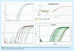
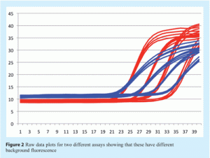
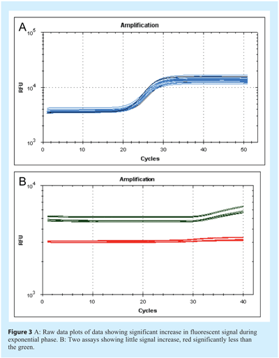
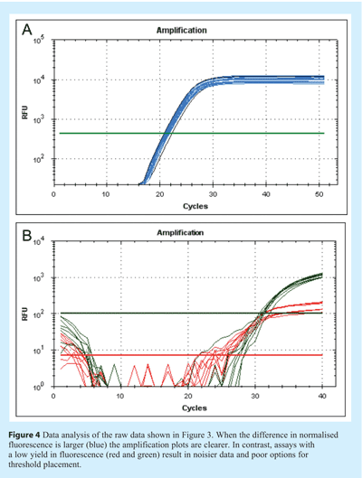
The physical appearance of the amplification plot provides an initial indication of assay quality. Initially, a little experience is required to develop familiarity with the fluorescent scale units used by the instrument. Examine the choice of values for Y axis scale, which denotes fluorescence: instruments are different and the absolute values will differ between them (see Figure 1). The initial focus for data analysis should be on the raw fluorescence values, the baseline settings, the threshold (if used) and melt curves (e.g. for SYBR Green I, Molecular Beacons or Scorpions). Analysis of the raw data reveals whether the fluorescence intensity range is appropriate. The raw signal in the region of exponential amplification used to determine the quantification cycle (Cq)1 must be well above background and well below saturation to avoid problems of spiking and poor signal uniformity. However, raw fluorescent data must be analysed further to eliminate inter-instrument variability and ensure that Cq values can be directly compared (see Figure 2). One approach is to subtract the background signal from all traces such that all baseline data are set at zero (dR). To do this the software must identify the data that constitute the background noise prior to genuine amplification. Figure 3 shows data prior to baseline normalisation and Figure 4 shows data after baseline normalisation. The significant increase in fluorescence during exponential amplification (blue trace) results in amplification plots that can be analysed, whereas the low signal data from the red traces results in normalised data that are spiky due to a low signal to noise ratio. Various algorithms are available for baseline normalisation and the most powerful are those that examine each amplification plot individually and set a baseline for each plot accordingly. In addition it is useful to have an option for the user to modify these settings. In instruments which have uneven detection systems the data require further correction to compensate for differences in fluorescent intensities across the block. This correction is traditionally achieved by including a constant concentration of reference dye (e.g. ROX) and plotting the relative fluorescent intensity of the signal of interest to the constant reference dye against cycle number (dRn/ΔRn/RFU).

Setting the threshold

It is an interesting exercise (worth a moment’s consideration on an otherwise dull Friday afternoon) to construct a standard curve spanning around six logs dilution range, preferably with as little as one to five target copies in the highest dilution, then run a qPCR and read the Cq values recorded using the instrument’s automatic settings. Now position the threshold higher and then lower and take the Cq readings for each threshold setting. The setting of the threshold affects the Cq value, of course. Of greater importance than the absolute Cq values alone are the differences between the values for the different concentrations. Calculate the differences between subsequent dilution points for the different threshold settings. Are they identical? If the assay is well optimised and linear you will observe that the absolute values of the Cq vary with threshold setting but the relative Cq (ΔCq) remains almost identical. This is because the amplification plots for each dilution of sample are parallel and so the change in threshold affects each amplification plot to the same degree. However, assays are not always so reliable and examples are readily found of plots of higher dilution factors (higher Cq) having a different gradient to the amplification plots of the lower dilutions (lower Cq). In these cases the absolute setting of the threshold influences the quantity or relative quantity estimates for the data. The threshold should be set in the log phase of amplification and at a position where all amplification plots are parallel, with an awareness that quantification of those that are not parallel results in an unacceptably large error. It is essential to utilise a common-sense approach to the consideration of amplification efficiencies and problems resulting from ill-considered dilution curves. This is demonstrated in a publication criticising a peer-reviewed paper for reporting impossibly high amplification efficiencies and applying incorrect statistical analyses that call into question the reliability and relevance of the conclusions based upon these assays2. Most recently, instrument manufacturers such as BioRad have introduced alternative methods for data analysis. This include innovations such as those that apply a multi-variable, non-linear regression model to individual well traces and then uses this model to compute an optimal Cq value, attempting to avoid some of the problems discussed above. There are many algorithms in development and only time will tell whether they provide a reliable solution. Without some concept of reference, Cq values are of limited value due to the fact that they can change with buffering, primers, machines, fluorescent chemistry along with a multitude of other factors.

Extraction of Cq or quantity values

As described above, the Cq value alone is of limited use since the absolute value is entirely dependent upon the threshold setting within the same experiment and a range of other factors when experiments are compared. Hence there is usually little point in publishing a Cq value3; instead, for most studies the Cq value must be converted to a more informative unit of measurement. In some cases an estimate of the relative quantity of a target can be determined by examination of the difference in Cq values between samples analysed from the same qPCR run. As demonstrated above, this must be performed with care since the use of Cq differences assumes that amplification of all concentrations of target result in amplification plots that are parallel to each other and displaced along the X-axis in a manner proportional to the starting concentration. As an alternative, a serial dilution of target of known concentration or relative concentration can be used to calibrate the measurement of target concentration in test samples3,4.

Using either of these approaches alone to quantify a target in a sample could result in inaccurate data because they rely on a number of presumptions. These include assumptions of similar sample quality, that any degradation does not effect quantification, equal reverse transcription (RT) efficiency, absence or equal effects of inhibitors or reaction enhancers5, equal loading of gDNA or cDNA into the qPCR assay and equal PCR efficiency in each sample for each target. Since it is clear that none of these assumptions is necessarily valid, there must be a process to compensate for these variables.

Normalisation

Data normalisation aims to address some of the deficiencies listed above, and there are numerous different approaches, with new ones proposed all the time. Normalisation to total sample mass or volume is a legacy approach remaining from northern blotting techniques when gel loading and sample transfer to filter paper was validated by probing for rRNA or so-called housekeeping genes such as GAPDH, whose expression was assumed to be stable between individuals, experimental conditions or physiological states. While still used for RT-qPCR measurements, there are several disadvantage of measuring mRNA or miRNA levels relative to sample mass or volume. For example, in a comparison of samples of different origin e.g. tumour biopsies and normal tissue it is incorrect to assume that the same tissue mass contains similar cell numbers, or that the relative distribution of proliferating cells is equal. Normalisation against total RNA will underestimate the expression of target genes in the tumour biopsies. This approach may be more suitable when the samples are extracted using laser capture micro dissection and a precise number and similar cells are targeted; even then this approach is not ideal. A related technique, again reminiscent of northern blotting, is to normalise to DNA or RNA concentration. While measuring gene copy number relative to input DNA concentration is a perfectly valid approach, the situation is more complicated for transcript quantification. When RNA concentration is determined, the vast majority of the RNA component is ribosomal RNA (rRNA). Transcription of rRNA is independent of the transcription of messenger RNA (mRNA) since it is transcribed by different enzymes. Furthermore as rRNA makes up ~80 % of the RNA fraction, normalisation to rRNA would mask subtle changes in the mRNA component; which typically comprises 2-5%. In addition, this approach does not take into account variations in the template RNA quality, or changes in rRNA levels dependent on cellular differentiation/proliferation status. Nonetheless, while not ideal, there may be situations where there are no other alternatives but to measure relative to total RNA and some analysis packages such as GenEx software from MultiD6 allow the total RNA concentration to be evaluated as a normalisation technique alongside other approaches. One theoretical solution would be to purify mRNA and normalise against total mRNA. Unfortunately the purification process introduces inaccuracies and an extra processing step that is undesirable and in many cases the biopsy is too small to allow efficient purification of re mRNA. A very common approach to correct for sample differences is to express the target concentration relative to that of a single internal reference gene. In order for this approach to be valid the expression of the single reference gene must remain constant between all experimental samples. To find such a convenient target additional validation is necessary, yet even today the all too common and misguided approach is to select this gene at random without validation; GAPDH, b actin and 18S are particular favourites in the published literature, usually used without validation or justification. When the reference gene is not stably expressed between all samples, a ratio of the target gene of interest to the reference gene will reflect the expression changes of both targets. This is unhelpful when the expression behaviour of neither target has been defined and can lead to inaccuracies and false results7. An amendment to this approach is to validate the chosen reference gene8 or select a significant reference gene with defined biology where the transcriptional response is well characterised (an approach referred to as normalisation to a Specific Internal Reference, or SIR). In this way the biology of the target gene is expressed relative to the change in biology of the reference gene. The problem with using these single reference gene approaches is that their resolution (minimum confident measurement) is limited to the minimum error of the technique.

An alternative approach, which is the current gold standard, is to express the data relative to the behaviour of multiple reference genes and use geometric averaging to measure and control for error induced trends in the relative reference gene expression. There are various approaches such as those offered by geNorm or Normfinder10,11 that allow the quantity of potential reference genes to be compared in selected groups of experimental and control samples. These use the combined variation of several genes to produce a stable reference factor for normalisation. However, the requirement for multiple reference transcript measurements, while very accurate and potentially providing 0.5 fold resolution12, is taxing on time, sample and resource. Furthermore, the use of single reference gene, SIR or multiple reference genes requires appropriate validation. A recent development points towards a possible solution to this conundrum. This method normalises the expression of the target gene of interest to several hundred different transcripts by targeting their embedded expressed ALU Repeats (EARs) in primate systems or B-Element Expressed Repeats (in mouse models). This avoids the problems associated with any bias caused by the use of a handful of genes, allows normalisation that is no longer tissue- or treatment-dependent and promises to increase data transparency and reproducibility. A similar approach can be used for the normalisation of microRNA expression, where the mean expression value of all expressed miRNAs in a given sample is used as a normalisation factor for microRNA real-time quantitative PCR data and is shown to outperform the current normalisation strategies in terms of better reduction of technical variation and more accurate appreciation of biological changes13.

Conclusions

Generation of qPCR data is deceptively simple, but once mastered the next challenge is to analyse the data so that they reflect the underlying biological or clinical phenomena, not technical the inadequacies. Appropriate data analysis and normalisation strategies are crucial aspects of the qPCR data analysis workflow, but are easily deflected by unsuitable approaches to this process. In order to reduce the risk of misinterpretation of qPCR data Sigma Aldrich has recently purchased GenEx software in order to give greater support to scientists during the data analysis process14. There are also commercial enterprises, such as MultiD6 or Biogazelle15, that provide a qPCR data analysis service using their own software, GenEx and qbaseplus, respectively. Use of such software makes it easier to analyse data properly, resulting in better quality publications and adds to, rather than confuses scientific progress.

References

1. S.A. Bustin, V. Benes, J.A. Garson, J. Hellemans, J. Huggett, M. Kubista, R. Mueller, T. Nolan, M.W. Pfaffl, G.F. Shipley, J. Vandesompele, and C.T. Wittwer, The MIQE Guidelines: Minimum Information for Publication of Quantitative Real-Time PCR Experiments. Clinical Chemistry 55 (2009) 609-620.
2. J.A. Garson, J.F. Huggett, S.A. Bustin, M.W. Pfaffl, V. Benes, J. Vandesompele, and G.L. Shipley, Unreliable real-time PCR analysis of human endogenous retrovirus-W (HERV-W) RNA expression and DNA copy number in multiple sclerosis. AIDS Res. Hum. Retroviruses 25 (2009) 377-378.
3. S.A. Bustin, and T. Nolan, Pitfalls of quantitative real-time reverse-transcription polymerase chain reaction. J Biomol Tech 15 (2004) 155-66.
4. Tania Nolan and Stephen A Bustin. Optimisation of the PCR step of a qPCR Assay. Eur Pharm Rev. 4 (2009) 15-20.
5. Huggett JF, Novak T, Garson JA, Green C, Morris-Jones SD, Miller RF, Zumla A. Differential susceptibility of PCR reactions to inhibitors: an important and unrecognised phenomenon. BMC Res Notes. 2008 Aug 28;1:70.
6. http://www.multid.se/genex.html
7. Dheda K, Huggett JF, Chang JS, Kim LU, Bustin SA, Johnson MA, Rook GA, Zumla A. The implications of using an inappropriate reference gene for real-time reverse transcription PCR data normalization. Anal Biochem. 2005 Sep 1;344(1):141-3.
8. Dheda K, Huggett JF, Bustin SA, Johnson MA, Rook G, Zumla A. Validation of housekeeping genes for normalizing RNA expression in real-time PCR. Biotechniques. 2004 Jul;37(1):112-4, 116, 118-9.
9. S.A. Bustin & J.F. Huggett (unpublished)
10. Vandesompele J, De Preter K, Pattyn F, Poppe B, Van Roy N, De Paepe A, Speleman F. Accurate normalization of real-time quantitative RT-PCR data by geometric averaging of multiple internal control genes. Genome Biol. 2002 Jun 18;3(7)
11. Andersen CL, Jensen JL, Ørntoft TF. Normalization of real-time quantitative reverse transcription-PCR data: a model-based variance estimation approach to identify genes suited for normalization, applied to bladder and colon cancer data sets. Cancer Res. 2004 Aug 1;64(15):5245-50.
12. J. Hellemans, O. Preobrazhenska, A. Willaert, P. Debeer, P.C. Verdonk, T. Costa, K. Janssens, B. Menten, N. Van Roy, S.J. Vermeulen, R. Savarirayan, W. Van Hul, F. Vanhoenacker, D. Huylebroeck, A. De Paepe, J.M. Naeyaert, J. Vandesompele, F. Speleman, K. Verschueren, P.J. Coucke, and G.R. Mortier, Loss-of-function mutations in LEMD3 result in osteopoikilosis, Buschke-Ollendorff syndrome and melorheostosis. Nat Genet 36 (2004) 1213-8.
13. P. Mestdagh, P. Van Vlierberghe, A. De Weer, D. Muth, F. Westermann, F. Speleman, and J. Vandesompele, A novel and universal method for microRNA RT-qPCR data normalization. Genome Biol 10 (2009) R64.
14. For further information email [email protected]
15. http://www.biogazelle.com