Real-time NIR monitoring of pharmaceutical blending processes with multivariate quantitative models

While industrial plant quality assurance and quality control (QA/QC) usually expect PAT data to be similar to those acquired during conventional laboratory type analysis, this may not always be efficient, convenient or possible. For instance, active pharmaceutical ingredient (API) assay may be one of the most critical quality attributes of a tablet in today’s QC. This generally requires quantification methodology to obtain a concentration value, usually reported in claim% or international units. With standard lab methods, such as high performance liquid chromatography (HPLC) or inductively-coupled plasma (ICP), quantification can be precise and accurate. However, these lab methods are time-consuming, expensive and require sample preparation with solvents that have associated monetary and ecological costs. Significant cost- and time-savings can be achieved with PATs. However, the challenge is to reach the same level of precision and accuracy with PATs as with conventional laboratory methods.

PAT usually generates an amount of data much larger than standard lab methods. Thus, even when the error of the PAT method is larger than with its lab counterpart, the level of control may be much greater because the amount of data acquired is more representative of the whole production batch. By acquiring, for example, more than 30 quality assessments with a PAT, it will be possible to establish whether the unit operation behaves normally and delivers as expected or if the process has biases or undesired deviations from controlled trajectories. Having more than 30 powder samples for every batch and quantifying each API in every sample is almost unthinkable for current QA/QC operations, but could be done with PAT.

Moreover, PAT quality assessment error could be lowered by applying alternative criteria. For instance, drug in-process QC may not always require determination of the amount of deviation, if such a deviation occurs; in many cases, it may only be necessary to identify if such a deviation is encountered. This can be done with qualitative models. By scanning homogeneous and within-specification samples of a formulation, it is possible to establish a reference model. Every data acquisition that enters the confidence interval of this reference model is determined to be within specifications and every one outside is considered out-of-specifications. The error of such a qualitative model can be small by adequate confidence intervals, and the sensitivity and accuracy of the methods can be ascertained with negative and positive testing studies, which may be a viable approach for many PATs.

Qualitative chemometrics for blend homogeneity analysis has been investigated in the first part of this work¹. Different qualitative analyses of a near-infrared (NIR) spectrum were applied to the V-blender mixing operation of a Wyeth multivitamin formulation with 16 ingredients, and were compared with lab results of thief samples acquired during each lot. Such a qualitative approach included (a) spectral variance and (b) distance from reference analyses. In the (a) case, the variance of consecutive spectra was monitored until a state of low and stable variance was achieved; this minimal variance was attributed to a state of blend uniformity. The latter computed a unitless distance value between the spectrum acquired during the mixing operation and a group of spectra said to be homogeneous or in-control. When the distance value of the lot-acquired sample was within a specified confidence interval, the lot was said to have reached homogeneity.

Many other studies of qualitative chemometrics were performed for blend analysis by near-infrared spectroscopy (NIRS)^2-5. However, most investigations conducted for the development of NIRS rely on quantitative chemometrics to assess the homogeneity or control state of the mix. Some investigate the monitoring of a tracer in a formulation by developing a quantitative model for this tracer. Berntsson et al.⁶ undertook such an analysis in a 2-component mixture for both small-scale (10dm³) and large-scale (3m³) Nauta mixers. Popo et al.⁷ also investigated the quantification of a tracer in a 2-component mixture in a laboratory scale V-blender (4qt) unit operation by NIR. The adequacy of their model was confirmed by standard laboratory QA UV spectroscopy analysis.

In Part 3 of their study, El-Hagrasy and Drennen⁸ investigated the monitoring of a tracer in a 2-component mixture and compared different types of chemometric regressions, such as Partial Least Squares (PLS), Principal Component Regression (PCR) and Multi-Linear Regression (MLR) to achieve a quantification model. The results indicated efficient monitoring of the 7 and 11 wt% concentration of the tracer but did not prove as efficient for low 3 wt% concentration. These types of monitoring provide a more typical approach to QA since API concentration could be monitored and validated within targeted limits.

More complex monitoring of ingredients in a pharmaceutical mixing operation was investigated by Bynum et al.⁹. In this case, all five components of the pharmaceutical formulation were quantified by PLS model development from lab samples with known gravimetric concentrations. The model was tested to follow the in-line concentrations of each component in a 20-L bin-blender.

The present study, conducted by the Université de Sherbrooke in collaboration with the Technical Services of Wyeth Pharmaceuticals Montréal, was aimed at investigating chemometric models for blend homogeneity assessment by NIR as a PAT tool. The results of qualitative analyses were reported in the first part¹. This second part focuses on quantitative analysis with chemometrics. A comparison of all methods will be reported in the Conclusion section.

Experimental set-up

In the present study, a model was built from lab-scale batches of the formulation using a 1-ft3 V-blender, and was scaled-up to analyse a 125-ft3 V-blender commercial batch. The experimental setup and methodology (Sections 2 and 3) were described in Part 1 of our study¹. However, they are reported here for continuity purposes.

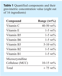
The formula investigated is a Wyeth proprietary multivitamin formulation containing 16 different ingredients, each having a concentration ranging from under 1wt% to more than 40wt%; the exact formulation is proprietary information, but a quick overview of it appears in Table 1. Notice that the first eight ingredients comprise over 75wt% of the total formulation. Consequently, several ingredients have considerably low concentrations (under 1wt%) and may not be visible with the sensitivity provided by the NIR system used.

The NIR system is a Micro-Electro-Mechanical System (MEMS)-based spectrometer that provides spectral coverage of 1,350 to 1,800nm and an acquisition time of less than 100ms. The measuring probe has a 40mm spot size, and sample penetration is estimated to be about 1 mm. The instrument is installed directly on the V-blender, and a sapphire window is mounted on its cover to provide a sampling port for the NIR probe to perform reflectance measurements. The system communicates with a laptop computer through a Wi-Fi wireless connection and can be trigger-operated to automatically acquire a NIR spectrum at a specified point in the rotation time-space. The trigger activates NIR acquisition when the blender is upside down with powder fully blanketing the V-blender’s cover. The powder is considered to be in a static state when powder analysis is performed. Each rotation triggers an acquisition, and each acquisition generates four NIR spectra averaged in a single spectrum for a total acquisition time of 400ms, excluding software integration. This averaging helps in increasing the signal-to-noise ratio.

Methodology

To best model a typical production batch, laboratory 1-ft³ scale batches in this study were used under the same operating conditions (manufacturing procedure) as the production batches with the exception that no side-mixing was done at lab scale. Thus, all vitamin ingredients were added to the V-blender separately, creating a maximum state of segregation before any mixing.

Experimental runs were performed according to the following protocol: A first batch with a mixing time of 15 minutes was produced and monitored with NIR technology. A preliminary blending curve was established with simple qualitative analysis. This analysis was used to set the two other blending times at 69s and 23s, respectively. The procedure was undertaken to ensure three batches with different homogeneity states. Since the 1-ft³ V-blender rotates at a speed of 26rpm, the number of rotations for each batch was 380, 30 and 10, respectively. The same number of spectra can be expected for each run. In the following pages, the three batches are referred to and reported by their run number:

• Run #1 = 15min blending time = 380 rotations;
• Run #2 = 69s blending time = 30 rotations;
• Run #3 = 23s blending time = 10 rotations.

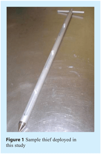
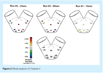
After the completion of each batch, a typical sample thief (see Figure 1) was used to acquire 10 samples at different locations of the V-blender’s volume. It is known that a thief sampling method can induce bias in the results^10,11, but this setup was selected as a reference because it is still generally accepted in production for blend homogeneity determination by most pharmaceutical manufacturers. The 10 sampling locations are shown in Figure 2. Each batch was discarded after sampling because it was assumed that sampling might remove considerable amounts of low-concentration ingredients in non-homogenized batches.

Each sample was scanned 10 times with the NIR system prior to any lab analysis; manual stirring was applied between each NIR data acquisition. The samples, acquired with the thief probe, were first poured on the acquisition window of the NIR spectrometer. A plastic stirrer was used to mix the powder sample between scans. The vitamin blend was visually heterogeneous; thus, static charge error was assumed to be negligible when compared to the obvious non-homogeneity.

After five scans, the sample was transferred back to the bottle, shaken manually and then poured again on the NIR sampling window for five more scans. The same acquisition parameters were used as the ones from the blend analyses. The chemometric quantitative model was built with these scans.

The samples were then sent to the QA Vitamin Laboratory of Wyeth Pharmaceuticals where the eight targeted ingredients were quantified by standard lab methods such as HPLC, ultra performance liquid chromatography (UPLC) or ICP.

The sample was also exposed to noise that may be encountered during production, such as particle attrition and static build-up. The inconvenience is that concentrations of the samples scanned cannot be planned. Also, this methodology does not guarantee that the concentration of ingredients between each sample will be linearly independent or uncorrelated.

The three blending lots were designed to alleviate these problems. By sampling a batch that should have achieved homogeneity (run #1), many samples should have the concentration of gravimetric values. Likewise, by sampling batches far from homogeneity (run #2 and run #3), many samples should have very distinct concentrations. The hypothesis is that by sampling a total of 30 samples out of three lots with different homogeneity states, the concentration distribution should be close to normal distribution. Moreover, to reduce the effect of co-linearity between concentrations of the samples, chemometrics analyses were restricted to bilinear models such as Principal Components Analysis (PCA) and PLS, which are known to perform better than regular models (such as MLR) in these conditions¹².

The thief sample locations can be seen in Figure 2. They are numbered from 1A to 5B. This figure illustrates the lab results for Vitamin C. The trend shown in Figure 2. is typical, and it was observed for each quantified component. For each batch and for each component, mass balance closure was 100±5%. Consequently, it can be concluded that, statistically, the samples taken were representative of the whole batch.

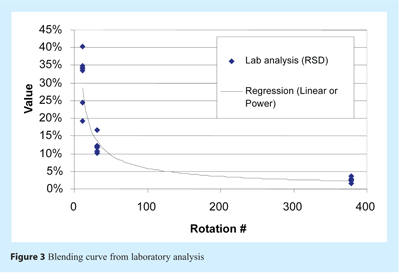
A lab blend curve was plotted with the Relative Standard Deviation (RSD) of concentrations for each component quantified and for each batch. The RSDs were then plotted versus the number of rotations to draw the blending curve (see Figure 3), which was used for lab reference homogeneity analysis. Regression can approximate the actual time required to achieve a homogeneous state where every component is below 5% RSD. However, the type of regression for optimal identification of the point where RSD values go below 5% is unknown. With exponential regression, blending time estimated from lab analysis was 126 rotations, or four minutes 50s, but the blending curve may also be simply linear between run #2 and run #3 and then stable until the RSD values of run #1. In that case, the necessary blending time to reach an acceptable mixing time would be just below 50 rotations.

NIR quantitative results

After each of the three batches, 10 samples were acquired by the sample thief method for a total of 30 samples. These samples were first scanned 10 times with the NIR analyzer and then sent to the QC labs for quantitative analysis by current laboratory methods such as HPLC. These laboratory results were used to build the NIR quantitative model. Note that since each sample was scanned 10 times, 10 spectra corresponded to every concentration analysed by the laboratory. Also, the concentration of microcrystalline cellulose (MCC) was computed in this quantification model. Note, however, that this raw material was not quantified by current QA tests performed on the samples. Instead, the concentration of total calcium was tested for each sample, which was then reported in the MCC concentration. Indeed, the MCC in the study was composed of 35wt% of calcium, an inorganic unseen in the NIR region. The concentration of raw material as a whole is reported, and may affect the model error for this raw material.

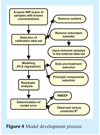
Quantification model building required very meticulous development because of the high complexity level. The large number of ingredients and the low concentration of some of them increase the complexity of the model and may lead to important errors. The process for model development is highlighted in Figure 4.

When building a quantitative model, two data sets are required. The data set used to calibrate regression will be called the calibration data set. The second data set to evaluate the error of the resulting model will be called the external data set. Even though 30 thief samples were acquired and quantified by lab methods, not all of them will benefit the model. Quantitative model building begins by selecting the calibration data set.

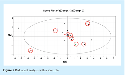
The first step of calibration data set selection consists of removing redundant samples. Samples that do not provide additional regression information will typically bias the index used to qualify the regression error and bias the weight of each data point in the regression. To do this redundancy analysis, PCA analysis can be performed on the Y-variables with unit-scaling pre-treatment. The unit-scaling process consists of removal of the mean of each variable and division by standard deviation. This pre-treatment allows us to scale the concentration values of each quantified vitamin or excipient so that they have the same weight and vary within the same range. Score 1 versus Score 2 plots can then spot samples that are repetitive. Figure 5 shows this redundant analysis in a t1 versus t2 score plot. In the figure, the samples that have been judged to be redundant are highlighted by a red circle. In such a case, one of the samples in the circle has been removed and included in the external data set.

Secondly, NIR scans that may be outliers must be removed to prevent them from introducing a bias in data pre-treatment and having too much weight on regression. This can be done by PCA analysis of X-variables of the samples without any data pre-treatments. The Hotelling T2 distance plot can spot outliers. Figure 6 shows this analysis for X-variables (the absorbance values of each NIR scan) of the calibration data set. Outliers can be spotted by a high distance value when compared to the distance value of scans from the same sample. Confidence intervals can discriminate outliers. In the case of our analysis, four scans were taken out as outliers. These scans were not included in the external data set. The decision to remove them was made after visual inspection of the spectra. They showed a clear difference from others of the same group. Several reasons could explain these outliers, but the most probable one was attributed to the trajectory segregation that may be encountered when pouring powder samples on the acquisition window. This is confirmed by the fact that most outliers are the first of a series of scans.

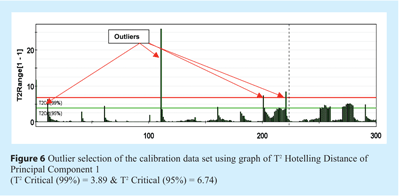
After these two steps, eight out of the 30 samples were removed, leaving 22 samples for the calibration data set. These eight samples were removed during redundancy analysis and, for the most part, were samples of run #1, as expected, since run #1 had the best uniformity. In outlier analysis, four single scans were removed.

The third step was regression and data pre-treatment comparative analysis. When performing data pre-treatment, a golden rule must be observed: the simpler the better. Data pre-treatment can dramatically change a data set so that any given performance can be obtained. However, too heavy and complex data pre-treatment may not perform well when the model is scaled-up from lab-scale to full-scale production. A Savitzsky-Golay first derivative over 15 points was selected in the course of analysis13. Note that these data pre-treatments were selected after extensive data pre-treatment analysis comparing many mathematical transformations and algorithms, such as Standard Normal Variate (SNV), Multiplicative Scatter Correction (MSC), 2nd derivative, unit variance, Pareto and their combinations. Model performance indicators were used to select the best data pre-treatment.

The model performance indicators selected were the following: Rx2, Q2, R2 and residual mean standard error of prediction (RMSEP) of each quantified component. Rx2 and Q2 are values that correspond to the goodness of fit of the PCA model with the raw data. A value close to one of these indicators means that the PCs selected for analysis adequately describe the raw data. More precisely, the Rx2 value is an indication of the goodness of fit between regression of the PCs and the raw data, and the Q2 value is an indication of the goodness of fit between regression of the PCs and the raw data as determined by cross-validation analysis. The Q2 value may be more relevant than the Rx2 value14.

The R2 and RMSEP indicators are values that correspond to the goodness of fit of the PLS regression model between X-variables (absorbance values) and Y-variables (concentration values). The R2 value is a typical regression fit between the concentration predicted by the model and the actual concentration. A R2 value close to one is desired. The RMSEP is calculated with the external data set as reference. The external data set consists of NIR scans of a sample with known concentrations that have not been used in the calibration data set. A good way to deal with the external data set is to employ the samples removed by redundancy analysis but more may be added. The concentrations of these references are then estimated by the model, and errors between the known and predicted concentrations are computed. This value may be the best indication of the actual prediction error for each component. A low RMSEP value is desired.

Analysis parallel to data pre-treatment analysis is the selection of the number of PCs. Selection of the number of PCs from PCA analysis is a complex operation. Typically, the software package will automatically select the number of PCs that result in the maximal Q2 value or minimal prediction error sum of squares (PRESS) value. However, this does not take the resulting RMSEP into account. One has to remember that the more PCs are selected, the better the Rx2 and R2 values will be. However, an excessive amount of PCs will result in modeling NIR noise and will thus decrease the Q2 and PRESS values and increase the RMSEP. In this study, selection of the PCs in each pre-treatment analysis was chosen to reflect an appropriate combination of the maximal R2 value and the minimal RMSEP for each component. Five PCs were sufficient for the PLS regression model to obtain good results for both indicators.

The last required analysis of a PLS model is residuals analysis. This analysis is required to spot possible outliers that may bias the results of the model once data pre-treatment and PCs have been computed. It can be conducted by looking at the PC1 versus PC2 score plot or the normal distribution curve. However, the removal of these outliers is a case-by-case study; obvious ones should be removed but extensive removal could discard important data variability. One basic criterion is that the data should follow a normal distribution plot. No spectra were removed in the course of this residual study.

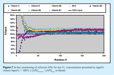
In Figure 7, the concentrations of eight of the 16 ingredients of the vitamin formulation are monitored for run #1, using the model developed, with the concentration data presented in % of input. Each point represents one spectrum and since a spectrum is acquired for each turn, 380 predictions are made for the 380 turns of run #1. In this graph, the concentrations are expected to stabilise near 100 input% and within a lower control limit (LCL) of 90% and an upper control limit (UCL) of 110%. In every case, the values seem to stabilise just over 105% instead of 100%, suggesting the presence of a small bias in the model. This may be due to the baseline effect difference from the spectra acquisition of thief samples with the spectra acquisition of run #1. However, this bias is considered acceptable since it is within the defined error (from RMSEP) of each prediction, as mentioned in Table 2.

It is interesting to observe the evolution of Vitamin C and Vitamin B3 concentrations since these two ingredients may have the best quantification sensitivity. It established that they vary quickly within the first 50 rotations, but stabilise after more than 100 rotations. This could be explained by the existence of two mixing mechanisms of different scale and speed. It was also observed with spectral variance and distance analysis from Part 1 of the study but it can be seen more clearly with this analysis. Thus, at the beginning, the prevailing mechanism would be fast dispersion by percolative diffusion of the ingredients within the moving bulk matrix, followed by a slower mechanism controlled by mass transfer between the moving blocks of bulk volume. Quantitative analysis suggests a blending time of at least 100 rotations. These two observations correspond well with the lab reference analysis.

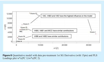
Even though some ingredients such as MCC, Vitamin B1 and B5 seem to have low RMSEP and adequate R2, when applied to run#1 lot scans in Figure 7, they seem to behave in a similar trend. These ingredients may be strongly correlated, which constitutes a disadvantage of the methodology used to develop this complex model. It can be seen in Figure 8 opposite, which presents the loading plot of the PLS model. The plot shows the contribution (weight) of each response variable (Y) to PC1 versus PC2. A value far from zero means that the Y-variable has a strong influence over the two main PCs. The graph confirms that these ingredients have a similar impact on the PCs and on the model. It was also observed that the correlated ingredients present similar strong absorption peaks in the NIR region investigated. Note, however, that the model employs five PCs, and the information of these ingredients may be better seen on other slightly less influential PCs.

NIR scale-up

A multivariate model developed in lab-scale experiments may perform well in laboratory trials but scale-up of the model is not always straight-forward. Ideally, a model should be developed with the NIR spectra acquired during a full-scale production batch so that every possible noise is taken into account in model building, knowing it is plausible that noises are a function of the unit operation scale. This is feasible when building qualitative distance analysis such as Part 1 of the study, but may be problematic when building a quantitative model. It was the case for the current study, and the model developed with laboratory scale data was used to monitor a full-scale production lot of the same formulation.

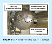
The same MEMS-based NIR system was fitted on a full-scale production V-blender with 125 ft3 of working volume. The probe of the system employed to acquire NIR spectra was fixed to a specially modified V-blender’s cover equipped with a sapphire window. Trigger acquisition was set for four spectra per turn averaged as one. See Figure 9 for more details.

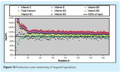
The batch monitored followed the regular manufacturing process of Wyeth Pharmaceuticals for the targeted formula. This includes two mixing steps in the V-blender: an initial mixing step of 20 minutes for every vitamin and mineral, and a second mixing step for lubricant addition. Note that the full-scale production process includes several premix operations performed in smaller blenders to better disperse low-concentration ingredients. This was not done with the lab-scale batches, and thus the blend curve was expected to differ slightly from the one in Figure 7.

The blend curve for the full-scale production batch appears in Figure 10, which shows the first 150 rotations of the final mix of ingredients, before lubricant addition. These rotations are considered representative of the actual blend curve expected for the initial mixing of all ingredients. Only 30 rotations seem sufficient to stabilise the mixing of ingredients, although a slow mixing process seems predominant until the last rotations. Analysis does confirm uniformity of the lot and the adequacy of mixing. Scale-up of the model seems adequate although it was unfeasible to compare actual production NIR scans with lab reference. Only a few of the ingredients actually stabilise around 100% of the theoretical input value. Even though scale-up of the model is adequate, the actual error of measurement is higher than the RMSEP values obtained in the lab scale study. This error was not measurable in the case of the production scale study. Moreover, the same kind of correlation is observed for low-concentration ingredients.

In this scale-up study, one could also wonder how a single scan could be representative of over one ton of powder being mixed in such a full-scale blender. It should be noted, however, that the amount of data collected by such a PAT is far greater that what can typically be acquired in blend studies, and thus the representation of a whole batch can be seen by many consecutive measurements instead of a single data point. This is the case in our study where homogeneity of the lot is considered not when all data points are within specifications, but only when all data points are within specifications during a sufficient amount of time. This amount of time should be determined through a historical study of several lots. Not performed here, it may be the subject of a future study. Homogeneity of the lot monitored and shown in Figure 10 is still considered adequate since all data points stabilise and never vary once stabilisation is observed.

Conclusion

A quantitative model for eight of the 16 ingredients of the targeted multivitamin formulation was developed at lab-scale with relatively low prediction errors. NIR technology can monitor batch homogeneity with a quantitative model at lab-scale or full-scale production. The results give significant insight into mixing mechanisms, but additional work is needed to link the observation with the physical phenomena occurring during mixing. Rigorous model development methodology is essential to prevent over-fitting and co-linearity of the variables in bi-linear models (i.e. PCA, PLS). The methodology was applied in the course of model development and was efficient for most targeted ingredients. The mixing trend resulting from the analysis clearly shows the targeted ingredients being mixed together and their stabilisation after only around 30 rotations. The ingredients reach their expected value within an anticipated prediction error, which may be slightly higher when the model is applied on full-scale production lots than on lab scale.

However, it was demonstrated that some low-concentration ingredients behaved in a similar trend, indicating a correlation between them. This was not seen in model prediction error evaluation (RMSEP) and correlation coefficient (R2) and highlights the complexity of developing such a model and ensuring that it performs adequately when applied on full-scale lots. The quantification precision of those low concentration ingredients is considered uncertain.

Given the high amount of effort required to build such a multivariate quantitative model and since the complexity of the model results in predictions that have a questionable error value, it is concluded that this type of analysis requires further improvement to answer QA needs in a regular pharmaceutical manufacturing process, especially when there is a need for predicting a large number of APIs or other ingredients as in multivitamin formulations. Even though the usual concentration value is achieved through this type of analysis, the errors may be much higher than what is expected in regular lab methods. Moreover, the analysis is formula-dependent and must be repeated for each formulation, or if a formulation is ever modified. One must remember that a model developed for one ingredient in a mix will have to be updated if the same ingredient is monitored in a different mix. Based on actual work observations, it can be said that the improvements required include: (a) the investigation of correlations existing between the concentrations of some ingredients, (b) the exploitation of data to reach a better understanding of mixing phenomena as a function of the ingredients’ properties, and (c) the study of particle physical effects on NIRS to better understand the noise that they may cause.

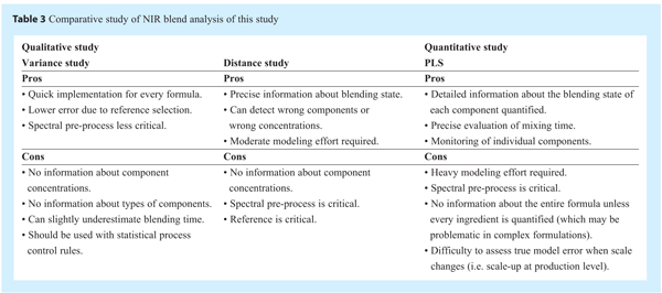
NIR technology is currently one of the most efficient tools for in-line process monitoring in the pharmaceutical industry because of its data acquisition speed and robust characteristics. As mentioned in Part 1 of this study, many other models may be applied on NIR spectra to acquire similar type of information without necessitating the actual concentration values of all targeted ingredients in a pharmaceutical formulation. These types of analysis may be more adequate for regular production, or one may decide to use the prediction from more than one type of model to alleviate the possible bias of one model in a particular lot, Table 3 presents a comparison of the proposed methods (pros and cons). The resulting PAT will be able to assess whether the mixing unit operation is in control, and it can be employed for continuous improvement or as part of a QbD initiative.

Acknowledgements

The authors are indebted to Wyeth Pharmaceuticals and the National Science and Engineering Research Council of Canada (NSERC) for funding related to this project. The scientific and technical contributions of the following fellows are gratefully acknowledged: Antoine Cournoyer (Wyeth Pharmaceuticals), Éliane Caron (Université de Sherbrooke), Carlo Benedetti (SNC-Lavalin Pharma), Guillaume Leonard (Université de Sherbrooke).

References

1. LAPOINTE-GARANT, P.-P., ABATZOGLOU, N., SIMARD, J.-S., Real-time NIR monitoring of a Pharmaceutical Blending Process through Multivariate Analysis-derived Models, WSEAS Proceedings, 2008.
2. EL-HAGRASY, A.S., DELGADO-LOPEZ M., DRENNEN, J.K., 3rd, A Process Analytical Technology Approach to Near-Infrared Process Control of Pharmaceutical Powder Blending. Part II: Qualitative Near-Infrared Models for Prediction of Blend Homogeneity, J. Pharm. Sci. 95(2) (2006) 407.
3. WOLD, S., ESBENSEN, K., GELADI, P., Chemom. Intell. Lab. Syst. 2 (1987) 37.
4. DE HASETH, J.A., AZARRAGA, L.V., Anal. Chem. 53 (1981) 2292.
5. BLANCO, M., GOZÁLEZ BAÑÓ, R., BERTRAN E., Monitoring Powder Blending in Pharmaceutical Processes by Use of Near Infrared Spectroscopy, Talanta 56 (2002) 203.
6. BERNTSSON, O., DANIELSSON, L.-G., LAGERHOLM, B., FOLESTAD, S., Quantitative In-line Monitoring of Powder Blending by Near Infrared Reflection Spectroscopy, Powder Technology 123(2) (2002) 185.
7. POPO, M., ROMERO-TORRES, S., CONDE, C., ROMAÑACH, R.J., Blend Uniformity Analysis Using Stream Sampling and Near Infrared Spectroscopy, AAPS PharmSciTech, Article 24, September 2002
8. EL-HAGRASY, A.S., DRENNEN, J.K. 3rd, A Process Analytical Technology Approach to Near-Infrared Process Control of Pharmaceutical Powder Blending. Part III: Quantitative Near-Infrared Calibration for Prediction of Blend Homogeneity and Characterization of Powder Mixing Kinetics, J. Pharm. Sci. 95(2) (2006) 422.
9. BYNUM, K., ZIELINSKI, J., PATEL, S., WABUYELE, B., LOBRUTTO, R., VIVILECCHIA, R., Blend Uniformity: A Mass Balance Approach, Am. Pharm. Rev. 10(6) (2007) 16, 18-22, 24-27.
10. BERMAN, J., PLANCHARD, J.A., Blend Uniformity and Unit Dose Sampling, Drug Dev. Ind. Pharm. 21(11) (1995) 1257.
11. PASTOR, R., GÓMEZ, R., BELLAMY, M., A Novel Sample Thief Design to Avoid Biased Data, Pharm. Techno. Yearbook 1 (1999) 1.
12. ESBENSEN, K., Multivariate Data Analysis – In Practice: An Introduction to Multivariate Data Analysis and Experimental Design, 5th edition, CAMO, Norway, 2004, 598 pages
13. SAVITZSKY, A., GOLAY, M.J.E., Smoothing and Differentiation of Data by Simplified Least Squares Procedures, Anal. Chem. 36 (1964) 1627.
14. ERIKSSON, L., JOHANSSON, E., KETTANEH-WOLD, N., WOLD, S., Multi- and Megavariate Data Analysis: Principles and Applications, Umetrics Academy, Sweden, 2001, 534 pages